The K-Nearest Neighbors (KNN) algorithm is a non-parametric learning algorithm, meaning that it does not assume anything about the underlying data. The idea behind KNN, proximity, is simple, yet it is capable of performing rather complex classifications. Let's talk about its theory.
The theory behind KNN
A simple example of how it works
Say we two classes of training data (red and blue), and the data points are scattered around a graph. One new data point is introduced at a random position of the graph. The (Euclidean/Manhattan) distances between the new data point and training points are calculated. Then any integer, k can be chosen to represent the number of nearest training data points. For that number of nearest data points, the newly introduced data point belongs to the class categorizing the most data points.
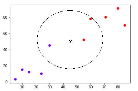
An example with k=3:
Credit: Scott Robinson
"X" is the newly introduced data point. Here you can see that with k=3, within the circle, there are 2 red training data points nearest to X and there is only 1 blue training data point. Therefore, the new data point is classified as red.
The good and bad of KNN
The good
Easy to understand and implement
KNN is a lazy learning algorithm, which means that it does not require any training to make real time predictions. This then makes KNN a relatively faster algorithm. New data can also be added seamlessly as a result.
Only 2 parameters are required for its implementation:
k-value
distance (either Euclidean or Manhattan)
The bad
Not good for high dimensional data. With increasing number of dimensions, it becomes increasingly difficult for the algorithm to calculate distance in each of the dimensions.
High prediction cost for large datasets arising from higher cost of distance calculation.
Not good for classification of categorical features. Methods of calculating distance other than Euclidean and Manhattan may be needed to apply KNN to categorical features. A discussion about it on Stack Overflow.
How to use the Python Scikit-learn library for KNN classfication
I used Jupyter Notebook to execute the necessary code as observed from this excellent tutorial. I made sure to make my code description as concise as possible.
1
2
3
4
5
# to import the necessary libraries

import numpy as np
import matplotlib.pyplot as plt
import pandas as pd
1
2
3
4
5
6
7
8
# to set the url of the famous iris dataset source
url = "https://archive.ics.uci.edu/ml/machine-learning-databases/iris/iris.data"

# to make a list of column names to be assigned to dataframe
names = ['sepal-length', 'sepal-width', 'petal-length', 'petal-width', 'Class']

# to read dataset to a pandas dataframe
dataset = pd.read_csv(url, names=names)
1
2
# to see the top 5 rows of "dataset"
dataset.head()
sepal-length
sepal-width
petal-length
petal-width
Class
0
5.1
3.5
1.4
0.2
Iris-setosa
1
4.9
3.0
1.4
0.2
Iris-setosa
2
4.7
3.2
1.3
0.2
Iris-setosa
3
4.6
3.1
1.5
0.2
Iris-setosa
4
5.0
3.6
1.4
0.2
Iris-setosa
1
2
3
# now we want to split the dataset into its features and labels
X = dataset.iloc[:, :-1].values # assigns first 4 columns to X
y = dataset.iloc[:, 4].values # assigns the "Class" column to y
1
2
3
4
5
6
7
# to avoid over-fitting, we need to divide the dataset into TRAINING and TEST splits
# this would give us a better idea of how the KNN algorithm performs during the TESTING phase

from sklearn.model_selection import train_test_split

# this will split the dataset into 80% training data and 20% test data
X_train, X_test, y_train, y_test = train_test_split(X, y, test_size=0.20)
1
2
3
4
5
6
7
8
9
10
# it doesn't stop here # feature scaling should be done next so the features can be uniformly evaluated # feature scaling basically normalizes the features, enabling the gradient descent algorithm to converge faster from sklearn.preprocessing import StandardScaler
# to make predictions on our test data y_pred = classifier.predict(X_test)
1
2
3
4
5
6
7
# now we want to evaluate our algorithm's accuracy
from sklearn.metrics import classification_report, confusion_matrix
print(confusion_matrix(y_test, y_pred))
print(classification_report(y_test, y_pred))

# the result shows that the KNN algorithm was able to classify all 30 records
# in the test set with pretty high accuracy.
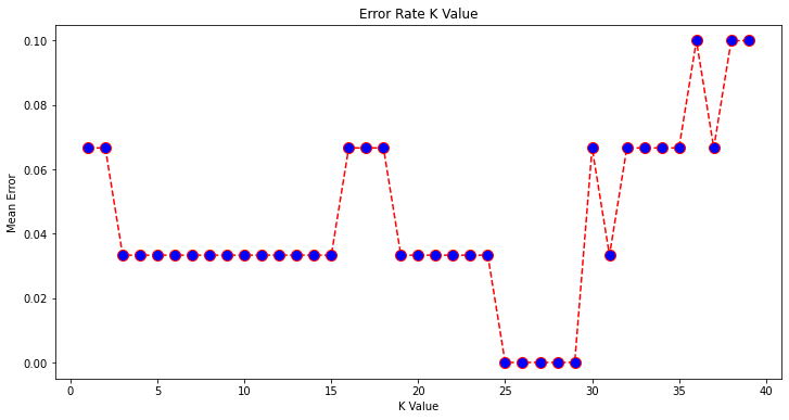
# so what if other k-values would provide us with better accuracy?
# one way to find out the best k-value is to plot the graph of k-value
# and the corresponding error rate

# let's now plot the mean error for the predicted values of test set for k-values
# from 1 to 40
error = []

# Calculating error for K values between 1 and 40
for i in range(1, 40):
    knn = KNeighborsClassifier(n_neighbors=i)
    knn.fit(X_train, y_train)
    pred_i = knn.predict(X_test)
    error.append(np.mean(pred_i != y_test))
1
2
3
4
5
6
7
# time to plot the error values against the k-values!
plt.figure(figsize=(12, 6))
plt.plot(range(1, 40), error, color='red', linestyle='dashed', marker='o',
         markerfacecolor='blue', markersize=10)
plt.title('Error Rate K Value')
plt.xlabel('K Value')
plt.ylabel('Mean Error')
Text(0, 0.5, 'Mean Error')
1
2
3
4
5
6
7
8
# we can see that the mean error is zero for k-values 25 to 29! # let's try k=27 and see what we get!
We now know that while any k-value can be chosen to deliver a decent result, one can always make a plot of mean error against k-values to further assess the effectiveness of certain k-values. This would then enable us to get an even more accurate classification result.
Even though the idea behind KNN is simple, the prediction power it offers is pretty simple. In fact, prediction making is one of the most challenging aspects of machine learning.
Leaning something new by first understanding something simple has definitely helped kept my interest alive for machine learning. I certainly hope you would feel the same way too. Shoutout to Scott Robinson for his amazing tutorial, which will be linked below.